Plotting for results

This notebook produces all results plots. It generates some gap in the data, fill with a method (filter, MDS …), compute metrics and then makes all relevant plots

%load_ext autoreload
%autoreload 2

import altair as alt

from meteo_imp.kalman.results import *
from meteo_imp.data import *
from meteo_imp.utils import *
import pandas as pd
import numpy as np
from pyprojroot import here
import torch
import seaborn as sns
import matplotlib.pyplot as plt
import matplotlib
from IPython.display import SVG, Image

from meteo_imp.kalman.results import _plot_timeseries, _get_labels
from functools import partial
from contextlib import redirect_stderr
import io

import polars as pl
from fastai.vision.data import get_grid
import cairosvg

the generation of a proper pdf is complex as altair_render doesn’t support XOffset, so plotsare first renderder to svg using vl-convert and then to pdf using cairosvg. However this last methods doesn’t support negative numbers …

Due to the high number of samples also cannot use the browser render in the notebook so using vl-convert to a png for the visualization in the notebook

import vl_convert as vlc
from pyprojroot import here
base_path_img = here("manuscript/Master Thesis - Evaluation of Kalman filter for meteorological time series imputation for Eddy Covariance applications - Simone Massaro/images/")
base_path_tbl = here("manuscript/Master Thesis - Evaluation of Kalman filter for meteorological time series imputation for Eddy Covariance applications - Simone Massaro/tables/")

base_path_img.mkdir(exist_ok=True), base_path_tbl.mkdir(exist_ok=True)

def save_show_plot(plot,
                   path,
                   altair_render=False # use altair render for pdf?
                  ):
    plt_json = plot.to_json()
    if not altair_render:
        svg_data = vlc.vegalite_to_svg(vl_spec=plt_json)
        with open(base_path_img / (path + ".svg"), 'w') as f:
            f.write(svg_data)

        cairosvg.svg2pdf(file_obj=open(base_path_img / (path + ".svg")), write_to=str(base_path_img / (path + ".pdf")))
    else:
        #save svg version anyway
        svg_data = vlc.vegalite_to_svg(vl_spec=plt_json)
        with open(base_path_img / (path + ".svg"), 'w') as f:
            f.write(svg_data)
        #convert to pdf using altair
        with redirect_stderr(io.StringIO()):
            plot.save(base_path_img / (path + ".pdf"))

    # render to image for displaying in notebook
    png_data = vlc.vegalite_to_png(vl_spec=plot.to_json(), scale=1)
    return Image(png_data)

reset_seed()
n_rep = 500

hai = pd.read_parquet(hai_big_path).reindex(columns=var_type.categories)
hai_era = pd.read_parquet(hai_era_big_path)

alt.data_transformers.disable_max_rows() # it is safe to do so as the plots are rendered using vl-convert and then showed as images

DataTransformerRegistry.enable('default')

Correlation

import matplotlib.pyplot as plt

import statsmodels.api as sm

def auto_corr_df(data, nlags=96):
    autocorr = {}
    for col in data.columns:
        autocorr[col] = sm.tsa.acf(data[col], nlags=nlags)
    return pd.DataFrame(autocorr)

auto_corr = auto_corr_df(hai).reset_index(names="gap_len").melt(id_vars="gap_len")
auto_corr.gap_len = auto_corr.gap_len / 2

auto_corr

	gap_len	variable	value
0	0.0	TA	1.000000
1	0.5	TA	0.998595
2	1.0	TA	0.995814
3	1.5	TA	0.992141
4	2.0	TA	0.987630
...	...	...	...
868	46.0	TS	0.959680
869	46.5	TS	0.961116
870	47.0	TS	0.962085
871	47.5	TS	0.962551
872	48.0	TS	0.962480

873 rows × 3 columns

p = (alt.Chart(auto_corr).mark_line().encode(
    x = alt.X('gap_len', title="Gap length [h]", axis = alt.Axis(values= [12, 24, 36, 48])),
    y = alt.Y("value", title="correlation"),
    color=alt.Color("variable", scale=meteo_scale, title="Variable"),
    facet =alt.Facet('variable', columns=3, sort = meteo_scale.domain, title=None,
                     header = alt.Header(labelFontWeight="bold", labelFontSize=20))
)
    .properties(height=120, width=250)
    .resolve_scale(y='independent', x = 'independent')
    .pipe(plot_formatter))

save_show_plot(p, "temporal_autocorrelation")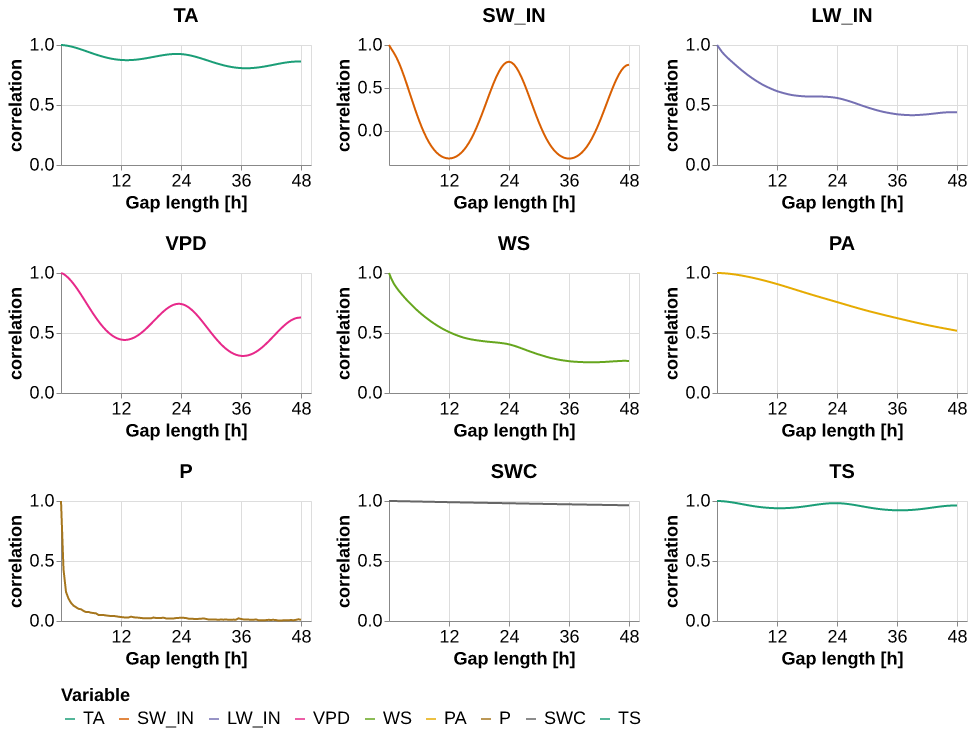

axes = get_grid(1,1,1, figsize=(10,8))
sns.set(font_scale=1.25)
sns.heatmap(hai.corr(), annot=True,     vmin=-1, vmax=1, center=0,
    cmap=sns.diverging_palette(20, 220, n=200), ax=axes[0], square=True, cbar=True)
# axes[0].set(xlabel="Variable", ylabel="Variable", title="Inter-variable Correlation");
# size_old = plt.rcParams["axes.labelsize"]
# w_old = plt.rcParams["axes.labelweight"]
# plt.rcParams["axes.labelsize"] = 30
# plt.rcParams["axes.labelweight"] = 'bold'
plt.tight_layout()
plt.xticks(weight = 'bold')
plt.yticks(weight = 'bold')

with matplotlib.rc_context({"axes.labelsize": 30}):
    plt.savefig(base_path_img / "correlation.pdf")
    plt.show()

# plt.rcParams["axes.labelsize"] = size_old
# plt.rcParams["axes.labelweight"] = w_old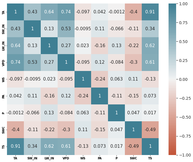

Comparison Imputation methods

base_path = here("analysis/results/trained_models")

def l_model(x, base_path=base_path): return torch.load(base_path / x)

models_var = pd.DataFrame.from_records([
    {'var': 'TA',    'model': l_model("TA_specialized_gap_6-336_v3_0.pickle",base_path)},
    {'var': 'SW_IN', 'model': l_model("SW_IN_specialized_gap_6-336_v2_0.pickle",base_path)},
    {'var': 'LW_IN', 'model': l_model("LW_IN_specialized_gap_6-336_v1.pickle",base_path)},
    {'var': 'VPD',   'model': l_model("VPD_specialized_gap_6-336_v2_0.pickle",base_path)},
    {'var': 'WS',    'model': l_model("WS_specialized_gap_6-336_v1.pickle",base_path)},
    {'var': 'PA',    'model': l_model("PA_specialized_gap_6-336_v3_0.pickle",base_path)},
    {'var': 'P',     'model': l_model("1_gap_varying_6-336_v3.pickle",base_path)},
    {'var': 'TS',    'model': l_model("TS_specialized_gap_6-336_v2_0.pickle",base_path)},
    {'var': 'SWC',   'model': l_model("SWC_specialized_gap_6-336_v2_1.pickle",base_path)},
])

@cache_disk(cache_dir / "the_results")
def get_the_results(n_rep=20):
    reset_seed()
    comp_Av = ImpComparison(models = models_var, df = hai, control = hai_era, block_len = 446, time_series=False)
    results_Av = comp_Av.compare(gap_len = [12,24, 48, 336], var=list(hai.columns), n_rep=n_rep) 
    return results_Av

results_Av = get_the_results(n_rep)

State of the art

the first plot is a time series using only state-of-the-art methods

reset_seed()
comp_ts = ImpComparison(models = models_var, df = hai, control = hai_era, block_len = 48+100, time_series=True, rmse=False)
results_ts = comp_ts.compare(gap_len = [48], var=list(hai.columns), n_rep=1) 

res_ts = results_ts.query("method != 'Kalman Filter'")
res_ts_plot = pd.concat([unnest_predictions(row, ctx_len=72) for _,row in res_ts.iterrows()])

scale_sota = alt.Scale(domain=["ERA-I", "MDS"], range=list(sns.color_palette('Dark2', 3).as_hex())[1:])

p = (facet_wrap(res_ts_plot, partial(_plot_timeseries, scale_color=scale_sota, err_band = False), col="var",
                y_labels = _get_labels(res_ts_plot, 'mean', None),
               )
            .pipe(plot_formatter)
    )
save_show_plot(p, "timeseries_sota", altair_render=True)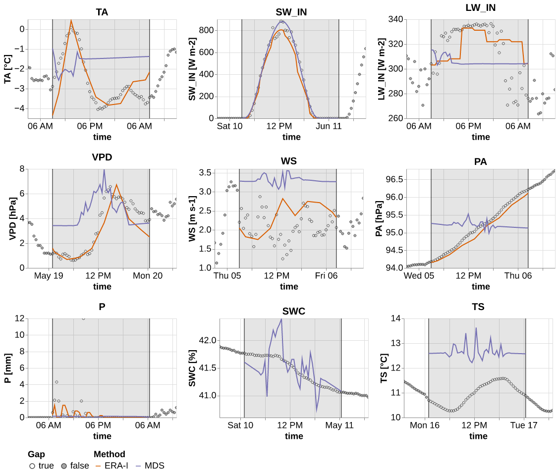

Percentage improvement

results_Av.method.unique()

['Kalman Filter', 'ERA-I', 'MDS']
Categories (3, object): ['Kalman Filter' < 'ERA-I' < 'MDS']

all_res = results_Av.query('var != "P"').groupby(['method']).agg({'rmse_stand': 'mean'}).T

all_res

method	Kalman Filter	ERA-I	MDS
rmse_stand	0.204628	0.307361	0.482837

percentage of improvement across all variables

(all_res["ERA-I"] - all_res["Kalman Filter"]) / all_res["ERA-I"] * 100 

rmse_stand    33.42398
dtype: float64

(all_res["MDS"] - all_res["Kalman Filter"]) / all_res["MDS"] * 100 

rmse_stand    57.619542
dtype: float64

res_var = results_Av.groupby(['method', 'var']).agg({'rmse_stand': 'mean'}) 

res_var = res_var.reset_index().pivot(columns='method', values='rmse_stand', index='var')

pd.DataFrame({'ERA': (res_var["ERA-I"] - res_var["Kalman Filter"]) / res_var["ERA-I"] * 100, 'MDS': (res_var["MDS"] - res_var["Kalman Filter"]) / res_var["MDS"] * 100 })

	ERA	MDS
var
TA	54.540802	77.713711
SW_IN	12.004508	35.516142
LW_IN	5.166063	52.289627
VPD	44.402821	65.407769
WS	21.064305	40.321732
PA	28.784191	90.751559
P	-18.544370	-22.084360
SWC	NaN	41.543006
TS	NaN	25.772326

res_var2 = results_Av.groupby(['method', 'var', 'gap_len']).agg({'rmse_stand': 'mean'}) 

res_var2 = res_var2.reset_index().pivot(columns='method', values='rmse_stand', index=['var', 'gap_len'])

pd.DataFrame({'ERA': (res_var2["ERA-I"] - res_var2["Kalman Filter"]) / res_var2["ERA-I"] * 100, 'MDS': (res_var2["MDS"] - res_var2["Kalman Filter"]) / res_var2["MDS"] * 100 })

		ERA	MDS
var	gap_len
TA	6	69.897582	85.052698
	12	58.766166	79.376385
	24	51.538443	75.395970
	168	41.823614	73.000401
SW_IN	6	9.519984	29.746651
	12	11.165399	30.639223
	24	14.232051	34.811941
	168	12.305658	42.651906
LW_IN	6	21.023524	59.136518
	12	9.110040	52.211404
	24	-3.553292	50.720632
	168	-4.260023	48.223005
VPD	6	66.980942	79.449579
	12	47.785633	69.081018
	24	33.663749	56.728120
	168	32.272332	57.702579
WS	6	32.402977	45.724043
	12	25.209162	43.275430
	24	15.543672	37.142502
	168	12.735569	36.436106
PA	6	39.823585	91.511486
	12	30.995845	90.532461
	24	24.727301	89.319180
	168	20.691181	91.421434
P	6	-18.485009	-13.917879
	12	-28.935358	-37.127331
	24	-24.423076	-29.998707
	168	-7.725322	-11.587796
SWC	6	NaN	61.302664
	12	NaN	47.976950
	24	NaN	42.535719
	168	NaN	23.301469
TS	6	NaN	64.264901
	12	NaN	46.699870
	24	NaN	27.050291
	168	NaN	-15.268479

Main plot

from itertools import product
import altair as alt

p = the_plot(results_Av)
save_show_plot(p, "the_plot")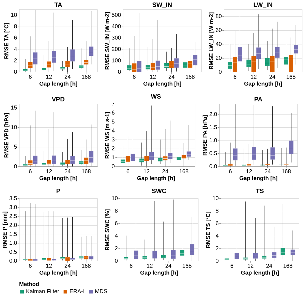

p = the_plot_stand(results_Av)
save_show_plot(p, "the_plot_stand")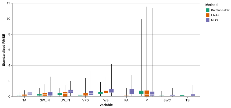

Table

t = the_table(results_Av)
the_table_latex(t, base_path_tbl / "the_table.tex", label="tbl:the_table",
                caption="\\CapTheTable")
t

		Kalman Filter		ERA-I		MDS
	RMSE	mean	std	mean	std	mean	std
Variable	Gap
TA	6 h	0.405453	0.258301	1.346910	0.997843	2.712546	1.896914
	12 h	0.606836	0.400849	1.471695	0.900611	2.942435	1.748131
	1 day (24 h)	0.741275	0.368468	1.529614	0.800256	3.012819	1.611311
	1 week (168 h)	1.020608	0.444591	1.754334	0.643160	3.780087	1.315472
SW_IN	6 h	44.636609	40.464629	49.333113	66.241975	63.536627	85.401585
	12 h	48.155186	33.868178	54.207691	49.769296	69.427115	68.936352
	1 day (24 h)	56.564277	30.042752	65.950367	40.930505	86.770917	59.603564
	1 week (168 h)	61.582820	25.740161	70.224393	34.883199	107.384249	53.606111
LW_IN	6 h	10.902409	7.736087	13.804628	12.987987	26.680077	15.022366
	12 h	13.421656	7.734502	14.766929	12.584725	28.085478	13.457335
	1 day (24 h)	14.593819	7.840046	14.093052	12.227900	29.614461	12.416763
	1 week (168 h)	17.062880	6.425136	16.365697	11.129569	32.954558	8.833972
VPD	6 h	0.428187	0.363168	1.296787	1.547397	2.083592	2.149288
	12 h	0.660623	0.504761	1.265213	1.288794	2.136626	2.095549
	1 day (24 h)	0.827563	0.501975	1.247527	1.032319	1.912472	1.605013
	1 week (168 h)	1.125680	0.633392	1.662069	1.127314	2.661345	1.965431
WS	6 h	0.616774	0.316972	0.912428	0.508295	1.136367	0.783146
	12 h	0.715412	0.350974	0.956550	0.524247	1.261203	0.796744
	1 day (24 h)	0.801851	0.343378	0.949427	0.446912	1.275665	0.608630
	1 week (168 h)	0.950211	0.363124	1.088887	0.348541	1.494891	0.615371
PA	6 h	0.045046	0.034294	0.074856	0.061726	0.530665	0.441476
	12 h	0.053359	0.041613	0.077328	0.058476	0.563603	0.427426
	1 day (24 h)	0.059481	0.038666	0.079021	0.051491	0.556899	0.404451
	1 week (168 h)	0.066325	0.047544	0.083628	0.053654	0.773143	0.384029
P	6 h	0.134093	0.274033	0.113173	0.315504	0.117710	0.305539
	12 h	0.178871	0.295419	0.138729	0.297227	0.130442	0.281377
	1 day (24 h)	0.206231	0.253588	0.165750	0.288432	0.158641	0.265257
	1 week (168 h)	0.239885	0.173820	0.222682	0.201782	0.214975	0.197499
SWC	6 h	0.508379	0.487342	NaN	NaN	1.313730	1.556829
	12 h	0.664855	0.471849	NaN	NaN	1.278001	1.323011
	1 day (24 h)	0.779066	0.640996	NaN	NaN	1.355740	1.472185
	1 week (168 h)	1.493784	0.947799	NaN	NaN	1.947605	1.488284
TS	6 h	0.341080	0.431992	NaN	NaN	0.954469	0.889126
	12 h	0.534363	0.783787	NaN	NaN	1.002555	0.876784
	1 day (24 h)	0.786670	0.851931	NaN	NaN	1.078373	0.856964
	1 week (168 h)	1.659875	1.077782	NaN	NaN	1.440008	0.764040

t = the_table(results_Av, 'rmse_stand', y_name="Stand. RMSE")
the_table_latex(t, base_path_tbl / "the_table_stand.tex", stand = True, label="tbl:the_table_stand", 
                caption = "\\CapTheTableStand")
t

		Kalman Filter		ERA-I		MDS
	Stand. RMSE	mean	std	mean	std	mean	std
Variable	Gap
TA	6 h	0.051164	0.032595	0.169965	0.125917	0.342294	0.239370
	12 h	0.076576	0.050583	0.185712	0.113647	0.371303	0.220595
	1 day (24 h)	0.093541	0.046497	0.193021	0.100984	0.380185	0.203330
	1 week (168 h)	0.128790	0.056103	0.221378	0.081160	0.477006	0.165998
SW_IN	6 h	0.218804	0.198354	0.241826	0.324711	0.311450	0.418630
	12 h	0.236052	0.166018	0.265721	0.243964	0.340325	0.337919
	1 day (24 h)	0.277272	0.147267	0.323282	0.200637	0.425342	0.292171
	1 week (168 h)	0.301873	0.126176	0.344233	0.170994	0.526387	0.262772
LW_IN	6 h	0.259855	0.184387	0.329028	0.309564	0.635910	0.358053
	12 h	0.319900	0.184349	0.351964	0.299952	0.669407	0.320751
	1 day (24 h)	0.347838	0.186865	0.335903	0.291448	0.705850	0.295949
	1 week (168 h)	0.406688	0.153141	0.390071	0.265269	0.785460	0.210555
VPD	6 h	0.098019	0.083135	0.296855	0.354224	0.476967	0.492006
	12 h	0.151227	0.115548	0.289627	0.295025	0.489108	0.479704
	1 day (24 h)	0.189442	0.114910	0.285579	0.236314	0.437795	0.367413
	1 week (168 h)	0.257686	0.144994	0.380474	0.258060	0.609224	0.449918
WS	6 h	0.379454	0.195008	0.561347	0.312715	0.699120	0.481810
	12 h	0.440138	0.215927	0.588492	0.322529	0.775922	0.490176
	1 day (24 h)	0.493318	0.211254	0.584110	0.274951	0.784819	0.374443
	1 week (168 h)	0.584592	0.223403	0.669909	0.214431	0.919692	0.378591
PA	6 h	0.052675	0.040103	0.087534	0.072180	0.620545	0.516250
	12 h	0.062397	0.048661	0.090425	0.068381	0.659061	0.499820
	1 day (24 h)	0.069556	0.045215	0.092405	0.060212	0.651223	0.472953
	1 week (168 h)	0.077558	0.055597	0.097793	0.062741	0.904092	0.449073
P	6 h	0.478431	0.977725	0.403790	1.125691	0.419979	1.090136
	12 h	0.638197	1.054031	0.494974	1.060481	0.465404	1.003928
	1 day (24 h)	0.735816	0.904779	0.591382	1.029100	0.566018	0.946414
	1 week (168 h)	0.855891	0.620173	0.794512	0.719941	0.767011	0.704660
SWC	6 h	0.057037	0.054677	NaN	NaN	0.147393	0.174667
	12 h	0.074593	0.052939	NaN	NaN	0.143384	0.148434
	1 day (24 h)	0.087407	0.071916	NaN	NaN	0.152106	0.165171
	1 week (168 h)	0.167594	0.106338	NaN	NaN	0.218510	0.166977
TS	6 h	0.060276	0.076342	NaN	NaN	0.168674	0.157127
	12 h	0.094433	0.138512	NaN	NaN	0.177172	0.154946
	1 day (24 h)	0.139021	0.150554	NaN	NaN	0.190571	0.151443
	1 week (168 h)	0.293335	0.190466	NaN	NaN	0.254479	0.135022

Timeseries

@cache_disk(cache_dir / "the_results_ts")
def get_the_results_ts():
    reset_seed()
    comp_Av = ImpComparison(models = models_var, df = hai, control = hai_era, block_len = 446, time_series=True, rmse=False)
    results_Av = comp_Av.compare(gap_len = [12,24, 336], var=list(hai.columns), n_rep=4) 
    return results_Av

results_ts = get_the_results_ts()

ts = plot_timeseries(results_ts.query("var in ['TA', 'SW_IN', 'LW_IN', 'VPD', 'WS']"), idx_rep=0)
save_show_plot(ts, "timeseries_1", altair_render=True)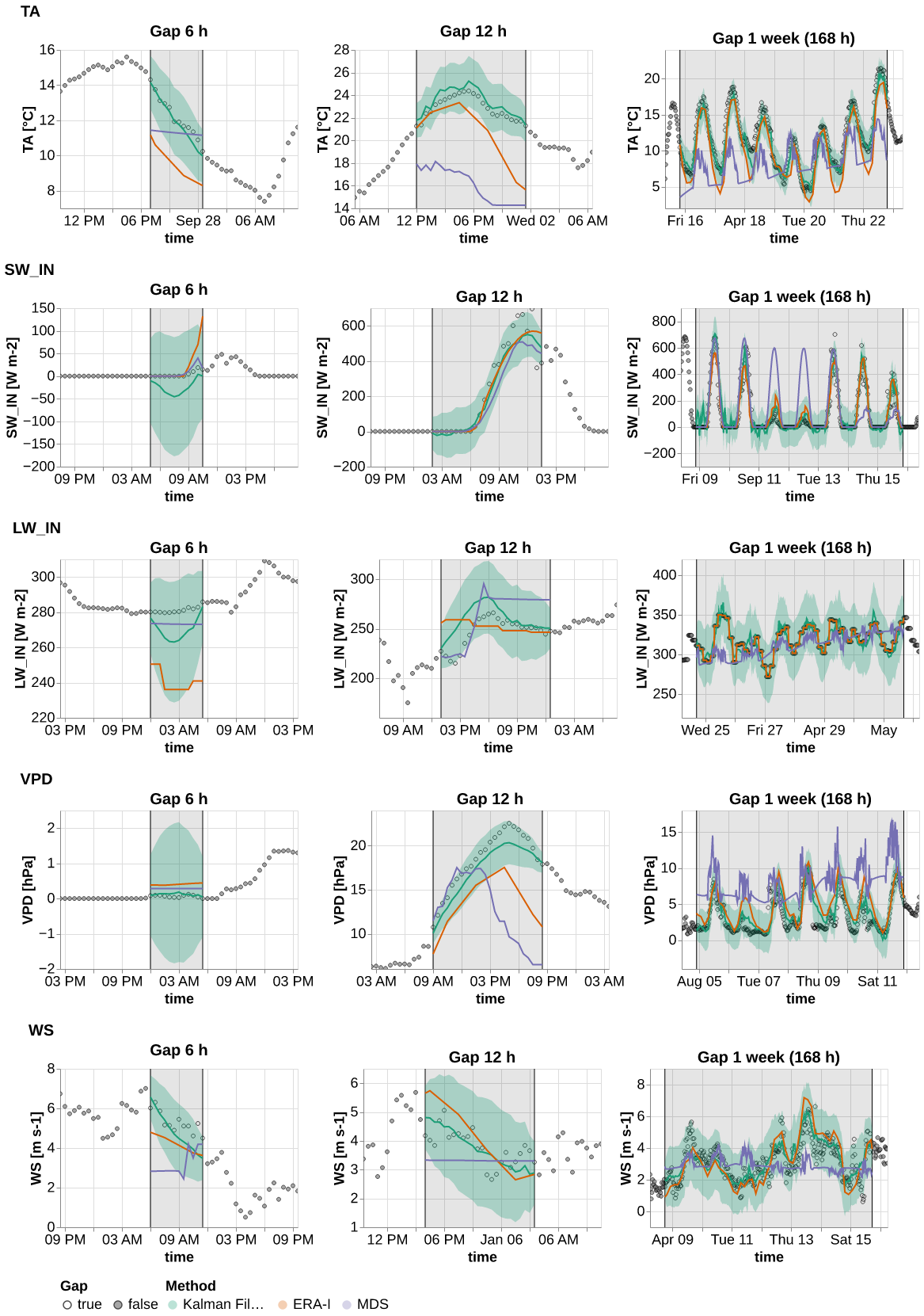

%time ts = plot_timeseries(results_ts.query("var in ['PA', 'P', 'TS', 'SWC']"), idx_rep=0)
%time save_show_plot(ts, "timeseries_2", altair_render=True)

CPU times: user 2.82 s, sys: 765 µs, total: 2.82 s
Wall time: 2.84 s
CPU times: user 9.53 s, sys: 127 ms, total: 9.66 s
Wall time: 12.8 s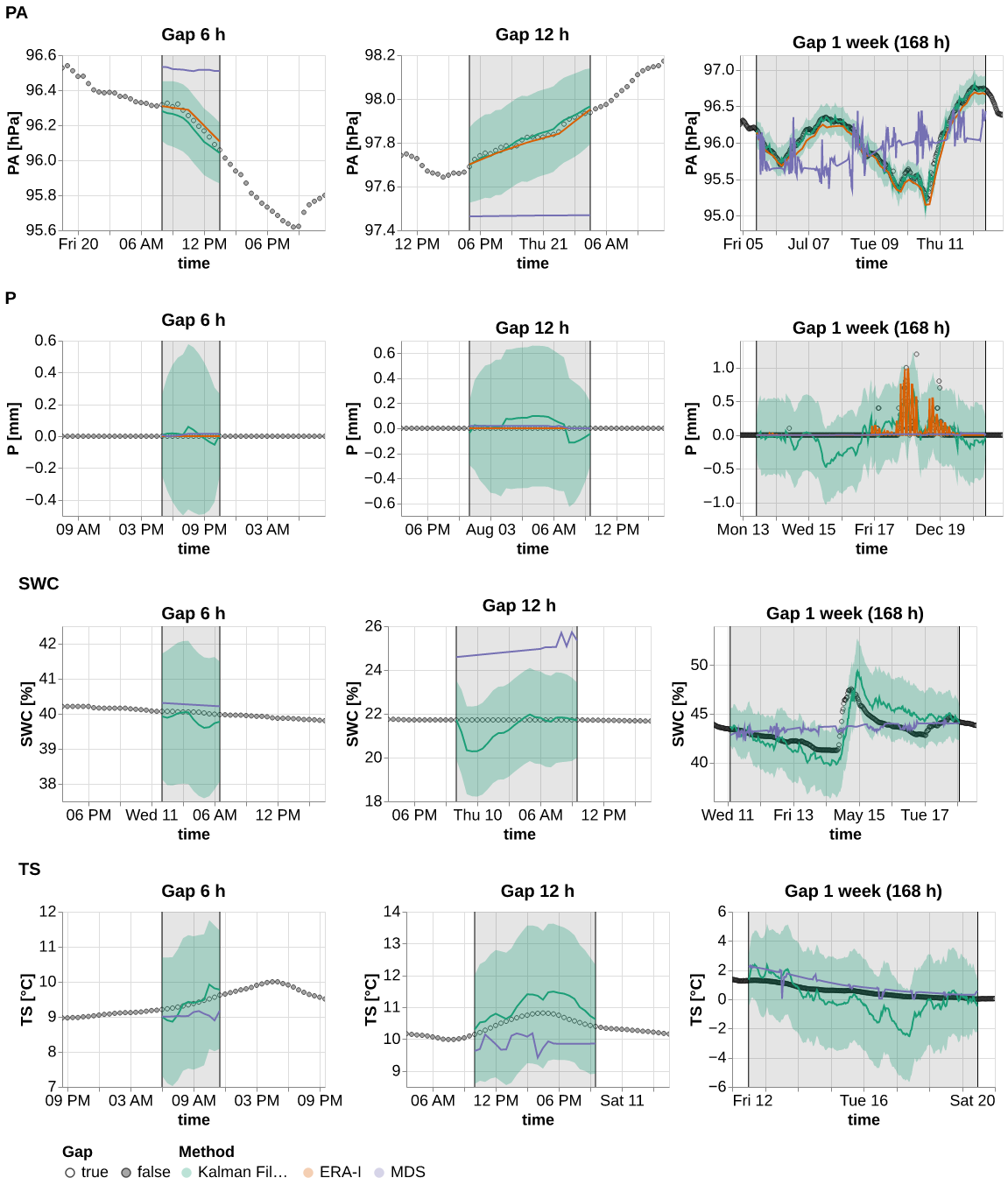

from tqdm.auto import tqdm

# @cache_disk(cache_dir / "ts_plot", rm_cache=True)
def plot_additional_ts():
    for idx in tqdm(results_ts.idx_rep.unique()):
        if idx == 0: continue # skip first plot as is done above
        ts1 = plot_timeseries(results_ts.query("var in ['TA', 'SW_IN', 'LW_IN', 'VPD', 'WS']"), idx_rep=idx)
        save_show_plot(ts1, f"timeseries_1_{idx}", altair_render=True)
        ts2 = plot_timeseries(results_ts.query("var in ['PA', 'P', 'TS', 'SWC']"), idx_rep=idx)
        save_show_plot(ts2, f"timeseries_2_{idx}", altair_render=True)        

plot_additional_ts()

Kalman Filter analysis

Gap len

@cache_disk(cache_dir / "gap_len")
def get_g_len(n_rep=n_rep):
    reset_seed()
    return KalmanImpComparison(models_var, hai, hai_era, block_len=48*7+100).compare(gap_len = [2,6,12,24,48,48*2, 48*3, 48*7], var=list(hai.columns), n_rep=n_rep)

gap_len = get_g_len(n_rep)

---------------------------------------------------------------------------
KeyboardInterrupt                         Traceback (most recent call last)
Input In [46], in <cell line: 1>()
----> 1 gap_len = get_g_len(n_rep)

File ~/Documents/uni/Thesis/meteo_imp/meteo_imp/utils.py:44, in cache_disk.<locals>.decorator.<locals>.new_func(*args)
     42 def new_func(*args):
     43     if tuple(args) not in cache:
---> 44         cache[tuple(args)] = original_func(*args)
     45         save_data()
     46     return cache[args]

Input In [45], in get_g_len(n_rep)
      1 @cache_disk(cache_dir / "gap_len")
      2 def get_g_len(n_rep=n_rep):
      3     reset_seed()
----> 4     return KalmanImpComparison(models_var, hai, hai_era, block_len=48*7+100).compare(gap_len = [2,6,12,24,48,48*2, 48*3, 48*7], var=list(hai.columns), n_rep=n_rep)

File ~/Documents/uni/Thesis/meteo_imp/meteo_imp/kalman/results.py:458, in KalmanImpComparison.compare(self, n_rep, gap_len, var)
    456 out = []
    457 for arg_set in tqdm(arg_sets):
--> 458     out.append(self._compare_single(**arg_set, n_rep=n_rep))
    459 return prep_df(pd.concat(out))

File ~/Documents/uni/Thesis/meteo_imp/meteo_imp/kalman/results.py:439, in KalmanImpComparison._compare_single(self, n_rep, gap_len, var)
    437 pred, targ, metric = imp.imp.preds_all_metrics(items = [items[i]], dls=dls, metrics=metrics_fn)
    438 pred, targ = pred[0], targ[0]
--> 439 pred = pred.mean.iloc[:, [var_idx]]
    440 targ = MeteoImpDf(targ.data.iloc[:, [var_idx]], targ.mask.iloc[:, [var_idx]], targ.control.iloc[:, [var_idx]])
    441 out = {
    442     'var': var,
    443     'loss': metric['loss'][0].item(),
   (...)
    446     'idx_rep': i,
    447 } | imp.drop(index=["model", "imp"]).to_dict()

File ~/.local/lib/python3.10/site-packages/pandas/core/indexing.py:140, in IndexingMixin.iloc(self)
    135 class IndexingMixin:
    136     """
    137     Mixin for adding .loc/.iloc/.at/.iat to Dataframes and Series.
    138     """
--> 140     @property
    141     def iloc(self) -> _iLocIndexer:
    142         """
    143         Purely integer-location based indexing for selection by position.
    144 
   (...)
    275         2  1000  3000
    276         """
    277         return _iLocIndexer("iloc", self)

KeyboardInterrupt: 

p = plot_gap_len(gap_len, hai, hai_era)
save_show_plot(p, "gap_len")

t = table_gap_len(gap_len)
table_gap_len_latex(t, base_path_tbl / "gap_len.tex", label="gap_len",
                caption="\\CapGapLen")
t

g_len_agg = gap_len.groupby('gap_len').agg({'rmse_stand': 'mean'})
(g_len_agg.iloc[0])/g_len_agg.iloc[-1]

g_len_agg = gap_len.groupby(['gap_len', 'var']).agg({'rmse_stand': 'mean'})
(g_len_agg.loc[1.])/g_len_agg.loc[168.]

g_len_agg

g_len_agg_std = gap_len.groupby('gap_len').agg({'rmse_stand': 'std'})
(g_len_agg_std.iloc[0])/g_len_agg_std.iloc[-1]

(gap_len.groupby(['gap_len', 'var']).agg({'rmse_stand': 'std'})
    .unstack("var")
    .droplevel(0, 1) 
    .plot(subplots=True, layout=(3,3), figsize=(10,10)))

# with open(base_path_tbl / "gap_len.tex") as f:
    # print(f.readlines())

Control

models_nc = pd.DataFrame({'model': [ l_model("1_gap_varying_336_no_control_v1.pickle"), l_model("1_gap_varying_6-336_v3.pickle")],
                          'type':   [ 'No Control',                                       'Use Control'                         ]})                                        

@cache_disk(cache_dir / "use_control")
def get_control(n_rep=n_rep):
    reset_seed()
    
    kcomp_control = KalmanImpComparison(models_nc, hai, hai_era, block_len=100+48*7)

    k_results_control = kcomp_control.compare(n_rep =n_rep, gap_len = [12, 24, 48, 48*7], var = list(hai.columns))
    
    return k_results_control

from time import sleep

k_results_control = get_control(n_rep)

k_results_control

p = plot_compare(k_results_control, 'type', y = 'rmse', scale_domain=["Use Control", "No Control"])
save_show_plot(p, "use_control")
p

from functools import partial

t = table_compare(k_results_control, 'type')
table_compare_latex(t, base_path_tbl / "control.tex", label="tbl:control",
                caption="\\CapControl")
t

Gap in Other variables

models_gap_single = pd.DataFrame.from_records([
    {'Gap':  'All variables', 'gap_single_var': False, 'model': l_model("all_varying_gap_varying_len_6-30_v3.pickle")},
    {'Gap':  'Only one var',  'gap_single_var': True,  'model': l_model("all_varying_gap_varying_len_6-30_v3.pickle")},
])

@cache_disk(cache_dir / "gap_single")
def get_gap_single(n_rep):
    kcomp_single = KalmanImpComparison(models_gap_single, hai, hai_era, block_len=130)

    return kcomp_single.compare(n_rep =n_rep, gap_len = [6, 12, 24, 30], var = list(hai.columns))

res_single = get_gap_single(n_rep)

p = plot_compare(res_single, "Gap", y = 'rmse', scale_domain=["Only one var", "All variables"])
save_show_plot(p, "gap_single_var")

t = table_compare(res_single, 'Gap')
table_compare_latex(t, base_path_tbl / "gap_single_var.tex", caption="\\CapGapSingle", label="tbl:gap_single_var")
t

res_singl_perc = res_single.groupby(['Gap', 'var', 'gap_len']).agg({'rmse_stand': 'mean'}).reset_index().pivot(columns = 'Gap', values='rmse_stand', index=['var', 'gap_len'])

pd.DataFrame({'Only one var': (res_singl_perc["All variables"] - res_singl_perc["Only one var"]) / res_singl_perc["All variables"] * 100})

res_singl_perc = res_single.groupby(['Gap', 'var']).agg({'rmse_stand': 'mean'}).reset_index().pivot(columns = 'Gap', values='rmse_stand', index=['var'])

pd.DataFrame({'Only one var': (res_singl_perc["All variables"] - res_singl_perc["Only one var"]) / res_singl_perc["All variables"] * 100})

Generic vs Specialized

models_generic = models_var.copy()

models_generic.model = l_model("1_gap_varying_6-336_v3.pickle") 
models_generic['type'] = 'Generic'

models_generic

models_var['type'] = 'Fine-tuned one var'

models_gen_vs_spec = pd.concat([models_generic, models_var])

models_gen_vs_spec

@cache_disk(cache_dir / "generic")
def get_generic(n_rep=n_rep):
    reset_seed()

    comp_generic = KalmanImpComparison(models_gen_vs_spec, hai, hai_era, block_len=100+48*7)

    return comp_generic.compare(n_rep =n_rep, gap_len = [12, 24, 48, 48*7], var = list(hai.columns))
k_results_generic = get_generic(n_rep)

plot_formatter.legend_symbol_size = 300

p = plot_compare(k_results_generic, 'type', y = 'rmse', scale_domain=["Fine-tuned one var", "Generic"])
save_show_plot(p, "generic")
p

t = table_compare(k_results_generic, 'type')
table_compare_latex(t, base_path_tbl / "generic.tex", label='tbl:generic', caption="\\CapGeneric")
t

res_singl_perc = k_results_generic.groupby(['type', 'var']).agg({'rmse_stand': 'mean'}).reset_index().pivot(columns = 'type', values='rmse_stand', index=['var'])

(res_singl_perc["Generic"] - res_singl_perc["Fine-tuned one var"]) / res_singl_perc["Generic"] * 100

Training

models_train = pd.DataFrame.from_records([
    # {'Train':  'All variables',  'model': l_model("All_gap_all_30_v1.pickle")  },
    {'Train':  'Only one var',   'model': l_model("1_gap_varying_6-336_v3.pickle")  },
    {'Train':  'Multi vars',     'model': l_model("all_varying_gap_varying_len_6-30_v3.pickle")  },
    {'Train':  'Random params',  'model': l_model("rand_all_varying_gap_varying_len_6-30_v4.pickle")  }
])

models_train

@cache_disk(cache_dir / "train")
def get_train(n_rep):
    reset_seed()
    kcomp = KalmanImpComparison(models_train, hai, hai_era, block_len=130)

    return kcomp.compare(n_rep =n_rep, gap_len = [6, 12, 24, 30], var = list(hai.columns))

res_train = get_train(n_rep)

res_train_agg = res_train.groupby(['Train', 'gap_len']).agg({'rmse_stand': 'mean'}).reset_index()

res_train_agg

p = plot_compare(res_train, "Train", y='rmse', scale_domain=["Multi vars", "Only one var", "Random params"])
save_show_plot(p, "train_compare")

t = table_compare3(res_train, 'Train')
table_compare3_latex(t, base_path_tbl / "train.tex", label="tbl:train_compare", caption="\\CapTrain")
t

Extra results

Standard deviations

hai_std = hai.std().to_frame(name='std')
hai_std.index.name = "Variable"
hai_std = hai_std.reset_index().assign(unit=[f"\\si{{{unit}}}" for unit in units_big.values()])

hai_std

latex = hai_std.style.hide(axis="index").format(precision=3).to_latex(hrules=True, caption="\\CapStd", label="tbl:hai_std", position_float="centering")

with open(base_path_tbl / "hai_std.tex", 'w') as f:
    f.write(latex)

Gap distribution

out_dir = here("../fluxnet/gap_stat")

site_info = pl.read_parquet(out_dir / "../site_info.parquet").select([
    pl.col("start").cast(pl.Utf8).str.strptime(pl.Datetime, "%Y%m%d%H%M"),
    pl.col("end").cast(pl.Utf8).str.strptime(pl.Datetime, "%Y%m%d%H%M"),
    pl.col("site").cast(pl.Categorical).sort()
])

def duration_n_obs(duration):
    "converts a duration into a n of fluxnet observations"
    return abs(int(duration.total_seconds() / (30 * 60)))

files = out_dir.ls()
files.sort() # need to sort to match the site_info
sites = []
for i, path in enumerate(files):
    sites.append(pl.scan_parquet(path).with_columns([
        pl.lit(site_info[i, "site"]).alias("site"),
        pl.lit(duration_n_obs(site_info[i, "start"] -  site_info[i, "end"])).alias("total_obs"),
        pl.col("TIMESTAMP_END").cast(pl.Utf8).str.strptime(pl.Datetime, "%Y%m%d%H%M").alias("end"),
    ]).drop("TIMESTAMP_END"))

gap_stat = pl.concat(sites)

pl.read_parquet(files[0])

gap_stat.head().collect()

def plot_var_dist(var, small=False, ax=None):
    if ax is None: ax = get_grid(1)[0]
    ta_gaps = gap_stat.filter(
        (pl.col("variable") == var)
    ).filter(
        pl.col("gap_len") < 200 if small else True
    ).with_column(pl.col("gap_len") / (24 *2 * 7)).collect().to_pandas().hist("gap_len", bins=50, ax=ax)
    ax.set_title(f"{var} - { 'gaps < 200' if small else 'all gaps'}")
    if not small: ax.set_yscale('log')
    ax.set_xlabel("gap length (weeks)")
    ax.set_ylabel(f"{'Log' if not small else ''} n gaps")
    # plt.xscale('log') 

plot_var_dist('TA_F_QC')

color_map = dict(zip(scale_meteo.domain, list(sns.color_palette('Set2', n_colors=len(hai.columns)).as_hex())))

qc_map = {
    'TA': 'TA_F_QC',
    'SW_IN': 'SW_IN_F_QC',
    'LW_IN': 'LW_IN_F_QC',
    'VPD': 'VPD_F_QC',
    'WS': 'WS_F_QC',
    'PA': 'PA_F_QC',
    'P': 'P_F_QC',
    'TS': 'TS_F_MDS_1_QC',
    'SWC': 'SWC_F_MDS_1_QC',
}

def pl_in(col, values):
    expr = False
    for val in values:
        expr |= pl.col(col) == val
    return expr

gap_stat.filter(pl_in('variable', qc_map.values())
               ).with_columns([
    pl.when(pl.col("gap_len") < 48*7).then(True).otherwise(False).alias("short"),
    pl.count().alias("total"),
    pl.count().alias("total len"),
]).groupby("short").agg([
    (pl.col("gap_len").count() / pl.col("total")).alias("frac_num"),
    (pl.col("gap_len").sum() / pl.col("total len")).alias("frac_len")
]).collect()

gap_stat.filter(pl_in('variable', qc_map.values())
               ).with_columns([
    pl.when(pl.col("gap_len") < 48*7).then(True).otherwise(False).alias("short"),
    pl.count().alias("total"),
    pl.count().alias("total len"),
]).groupby("short").agg([
    (pl.col("gap_len").count() / pl.col("total")).alias("frac_num"),
    (pl.col("gap_len").sum() / pl.col("total len")).alias("frac_len")
]).collect()

frac_miss = gap_stat.filter(
    pl_in('variable', qc_map.values())
).groupby(["site", "variable"]).agg([
    pl.col("gap_len").mean().alias("mean"),
    (pl.col("gap_len").sum() / pl.col("total_obs").first()).alias("frac_gap")
])

frac_miss.groupby('variable').agg([
    pl.col("frac_gap").max().alias("max"),
    pl.col("frac_gap").min().alias("min"),
    pl.col("frac_gap").std().alias("std"),
    pl.col("frac_gap").mean().alias("mean"),
]).collect()

frac_miss.sort("frac_gap", reverse=True).collect()

site_info.filter((pl.col("site") == "US-LWW"))

gap_stat.filter((pl.col("site") == "US-LWW") & (pl.col("variable") == "LW_IN_F_QC" )).collect()

import matplotlib

matplotlib.rcParams.update({'font.size': 22})
sns.set_style("whitegrid")

def plot_var_dist(var, ax=None, small=True):
    if ax is None: ax = get_grid(1)[0]
    
    color = color_map[var]
    var_qc = qc_map[var]
    ta_gaps = gap_stat.filter(
        (pl.col("variable") == var_qc)
    ).filter(
        pl.col("gap_len") < (24 * 2 *7) if small else True 
    ).with_column(pl.col("gap_len") / (2 if small else 48 * 7)
                 ).collect().to_pandas().hist("gap_len", bins=50, ax=ax, edgecolor="white", color=color)
    ax.set_title(f"{var} - { 'gap length <  1 week' if small else 'all gaps'}")
    ax.set_xlabel(f"Gap length ({ 'hour' if small else 'week'})")
    ax.set_ylabel(f"Log n gaps")
    ax.set_yscale('log') 
    plt.tight_layout()

vars = gap_stat.select(pl.col("variable").unique()).collect()

vars.filter(pl.col("variable").str.contains("TA"))

for ax, var in zip(get_grid(9,3,3, figsize=(15,12), sharey=False), list(var_type.categories)):
    plot_var_dist(var, ax=ax)
plt.savefig(base_path_img / "gap_len_dist_small.pdf")

for ax, var in zip(get_grid(9,3,3, figsize=(15,12), sharey=False), list(var_type.categories)):
    plot_var_dist(var, ax=ax, small=False)
plt.savefig(base_path_img / "gap_len_dist.pdf")

Square Root Filter

Numerical Stability

from meteo_imp.kalman.performance import *

err = cache_disk(cache_dir / "fuzz_sr")(fuzz_filter_SR)(100, 110) # this is already handling the random seed

p = plot_err_sr_filter(err)
save_show_plot(p, "numerical_stability")

Performance

@cache_disk(cache_dir / "perf_sr")
def get_perf_sr():
    reset_seed()
    return perf_comb_params('filter', use_sr_filter=[True, False], rep=range(100),
                           n_obs = 100,
                           n_dim_obs=9,
                           n_dim_state=18,
                           n_dim_contr=14,
                           p_missing=0,
                           bs=20 ,
                           init_method = 'local_slope'
                           ) 

perf1 = (get_perf_sr()
    .groupby('use_sr_filter')
    .agg(pl.col("time").mean())
    .with_column(
        pl.when(pl.col("use_sr_filter"))
        .then(pl.lit("Square Root Filter"))
        .otherwise(pl.lit("Standard Filter"))
        .alias("Filter type")
    ))

perf1

(perf1[0, 'time'] - perf1[1, 'time']) / perf1[1, 'time'] * 100

plot_perf_sr = alt.Chart(perf1.to_pandas()).mark_bar(size = 50).encode(
    x=alt.X('Filter type', axis=alt.Axis(labelAngle=0)),
    y=alt.Y('time', scale=alt.Scale(zero=False), title="time [s]"),
    color=alt.Color('Filter type',
                    scale = alt.Scale(scheme = 'accent'))
).properties(width=300)

save_show_plot(plot_perf_sr, "perf_sr")